In this post I’d like to discuss how finite fields (and more generally finite rings) can be used to study two fundamental computational problems in number theory: computing square roots modulo a prime and proving primality for Mersenne numbers. The corresponding algorithms (Cipolla’s algorithm and the Lucas-Lehmer test) are often omitted from undergraduate-level number theory courses because they appear, at first glance, to be relatively sophisticated. This is a shame because these algorithms are really marvelous — not to mention useful — and I think they’re more accessible than most people realize. I’ll attempt to describe these two algorithms assuming only a standard first-semester course in elementary number theory and familiarity with complex numbers, without assuming any background in abstract algebra. These algorithms could also be used in a first-semester abstract algebra course to help motivate the practical utility of concepts like rings and fields.
Anecdotal Prelude
In researching this blog post on Wikipedia, I learned a couple of interesting historical tidbits that I’d like to share before getting on with the math.
 The French mathematician Edouard Lucas (of Lucas sequence fame) showed in 1876 that the 39-digit Mersenne number
  is prime. This stood for 75 years as the largest known prime. Lucas also invented (or at least popularized) the Tower of Hanoi puzzle and published the first description of the Dots and Boxes game. He died in quite an unusual way: apparently a waiter at a banquet dropped what he was carrying and a piece of broken plate cut Lucas on the cheek. Lucas developed a severe skin inflammation and died a few days later at age 47.
Derrick Henry Lehmer was a long-time professor of mathematics at U.C. Berkeley. In 1950, Lehmer was one  of 31 University of California faculty members fired for refusing to sign a loyalty oath during the McCarthy era. In 1952, the California Supreme Court declared the oath unconstitutional, and Lehmer returned to Berkeley shortly thereafter. Lehmer also built a number of fascinating mechanical sieve machines designed to factor large numbers.
Rings and fields
Let  be an integer and let
  denote the set
  together with the operations of addition and multiplication modulo
  . Such a structure — a set together with two binary operations
  and
and  satisfying various axioms such as the associative, commutative, and distributive laws — is called a (commutative) ring. (Click here for a more detailed and formal discussion.) One of the axioms for a ring is that we can subtract any two elements, giving an inverse to the addition operation. If we can also divide by any nonzero element, giving an inverse to multiplication, then we call the ring a field. In this post we will be particularly interested in studying finite rings and fields.
The prototypical example of a finite field is  for
for  a prime number. We can also construct fields with
  elements by analogy with the complex numbers. Choose a non-square
  and define
 ![{\mathbf F}_p[\sqrt{d}]](https://s0.wp.com/latex.php?latex=%7B%5Cmathbf+F%7D_p%5B%5Csqrt%7Bd%7D%5D&bg=ffffff&fg=404040&s=0&c=20201002) to be the set of all formal expressions of the form
to be the set of all formal expressions of the form  with
with  , together with the addition and multiplication laws
  and
and  . One can easily check that is a field, with the reciprocal of
  given by
  , where
  and
and  . We can identify
  with the subfield
  of .
of .
Here are two basic properties of fields, both of which are usually known as “Lagrange’s Theorem”:
Lagrange #1: A polynomial of degree  with coefficients in a field
  can have at most
  roots in . (This is completely false if we replace “field” by “ring”.) See here for a proof in the special case
  which generalizes immediately to any field. We just need the following special case: the only roots of
  in are
  . This follows from the fact that
  in implies that either
  or
or  .
.
Lagrange #2: Let be a finite field with  elements and let
  denote the nonzero elements of . Then the order of any
  (defined as the smallest positive integer
  such that
  ) divides
  . (This can be viewed as an extension of Fermat’s Little Theorem, the proof is basically the same: multiplication by
  permutes the elements of , and thus
  . Hence
  . Writing
  with
with  integers such that
  , it follows that
  and hence
  .)
.)
The following property of the fields will be crucial in what follows.
Key Lemma: For ![\alpha \in {\mathbf F}_p[\sqrt{d}]](https://s0.wp.com/latex.php?latex=%5Calpha+%5Cin+%7B%5Cmathbf+F%7D_p%5B%5Csqrt%7Bd%7D%5D&bg=ffffff&fg=404040&s=0&c=20201002) , we have
, we have  .
.
Proof: Since  is a quadratic non-residue modulo , Euler’s Criterion tells us that
  in . Thus
  in . From the binomial theorem, the fact that
  in , and Fermat’s Little Theorem, it follows that
  as desired.
Computing modular square roots
We now turn to Cipolla’s algorithm for finding a solution to  when
when  is a nonzero square (quadratic residue) modulo the odd prime . If
  , one checks easily that the two solutions are
  , which can be efficiently computed via repeated squaring. However, the case
  cannot be treated in a similarly elementary and explicit way.
The first step in Cipolla’s algorithm is to find an integer  with
with  such that
  is not a square modulo . The only known method to do this efficiently is probabilistic: for a random value of , the number
  will be a non-square modulo with probability
  . Thus, if
  are chosen randomly, the probability that none of the
  works will be
  . So in practice, we will always very quickly be able to find a suitable value of , since for any particular
  we can efficiently decide whether or not is a square mod (using, for example, the Law of Quadratic Reciprocity for the Jacobi symbol).
Theorem 1: The two solutions in  to
to  (i.e., the two solutions to ) are
  .
.
Proof: Let  . Then
  , which by the Key Lemma equals
  Thus
Thus  are square roots of in . Moreover,
  , since by assumption the polynomial
  has two roots in , and it follows from Lagrange #1 that these are the only roots in the larger field .
We thus obtain:
Cipolla’s Algorithm: Let be a non-zero quadratic residue modulo . Compute  using repeated squaring in the finite field , where
  is a quadratic non-residue mod for some integer . The result is an element of whose square is equal to .
For computer implementation of this algorithm, it is useful to identify an element ![a+b\sqrt{d} \in {\mathbf F}_p[\sqrt{d}]](https://s0.wp.com/latex.php?latex=a%2Bb%5Csqrt%7Bd%7D+%5Cin+%7B%5Cmathbf+F%7D_p%5B%5Csqrt%7Bd%7D%5D&bg=ffffff&fg=404040&s=0&c=20201002) with ordered pair
with ordered pair  , just as a complex number is often identified with a point in the Euclidean plane. The addition law on ordered pairs is given by the rule
  and the multiplication law is given by
  .
.
We note, for use in the next section, that these addition and multiplication laws make sense on ordered pairs of integers modulo even if is not prime, or if is a square modulo . Abusing terminology somewhat, we denote the corresponding ring by ![({\mathbf Z} / n{\mathbf Z})[\sqrt{d}]](https://s0.wp.com/latex.php?latex=%28%7B%5Cmathbf+Z%7D+%2F+n%7B%5Cmathbf+Z%7D%29%5B%5Csqrt%7Bd%7D%5D&bg=ffffff&fg=404040&s=0&c=20201002) .
.
Primality proving for Mersenne numbers
We now turn to the problem of determining whether a large positive integer is prime. Though there are general algorithms for doing this (e.g. the celebrated polynomial-time test due to Agrawal, Kayal, and Saxena), such algorithms are much slower than special-purpose algorithms designed for numbers of a specific form. To illustrate our point, all of the largest known prime numbers are Mersenne numbers, meaning that they have the form  for some odd positive integer
  . More precisely, the largest number proven to be prime (as of November 2013) is the 17,425,170-digit Mersenne prime
  . It was discovered by the GIMPS project in January 2013. The reason that Mersenne numbers can be tested for primality in a particularly efficient way is because of the Lucas-Lehmer test, which we now describe.
We begin by observing that if is a Mersenne prime, then  is a quadratic residue modulo and
  is a quadratic non-residue modulo . This is a straightforward consequence of the Law of Quadratic Reciprocity, since one shows easily that
  and
and  .
.
Theorem 2: Let be a Mersenne number. Then is prime if and only if  in the ring
 ![({\mathbf Z} / n{\mathbf Z}) [\sqrt{3}]](https://s0.wp.com/latex.php?latex=%28%7B%5Cmathbf+Z%7D+%2F+n%7B%5Cmathbf+Z%7D%29+%5B%5Csqrt%7B3%7D%5D&bg=ffffff&fg=404040&s=0&c=20201002) .
.
Proof: Suppose first that  is prime. Let
  be a square root of in and let
  in the field
 ![{\mathbf F}_p[\sqrt{3}]](https://s0.wp.com/latex.php?latex=%7B%5Cmathbf+F%7D_p%5B%5Csqrt%7B3%7D%5D&bg=ffffff&fg=404040&s=0&c=20201002) . Then
. Then  and
and  . Conversely, suppose and let be a prime divisor of . Let
  if is a square mod , and let
 ![{\mathbf F} = {\mathbf F}_q [\sqrt{3}]](https://s0.wp.com/latex.php?latex=%7B%5Cmathbf+F%7D+%3D+%7B%5Cmathbf+F%7D_q+%5B%5Csqrt%7B3%7D%5D&bg=ffffff&fg=404040&s=0&c=20201002) otherwise. Since
otherwise. Since  but
but  , it follows that the order of
  in
in  is
is  . By Lagrange #2,
  divides
  , which is either
  or
or  . In either case,
  . Since this is true for all primes dividing , it follows that is prime.
Since one can compute  in the ring via repeated squaring, the theorem gives a practical method for testing Mersenne numbers for primality. However, there is a reformulation of the theorem which is more elementary and better suited to computer implementation; we describe this now. (We first note that the theorem remains true, with the same proof, if we replace by
  .)
.)
Let  , and recursively define a sequence
  of integers modulo by the rule
  and
and  for
for  . (In other words,
  where
where  is the
  iterate of
  .)
.)
Lucas-Lehmer Test: The Mersenne number with odd is prime if and only if  .
.
Proof: We first observe that 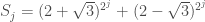 in for all
  : for
: for  this is clear, and a simple calculation shows that
If is prime, then  Thus
Thus  in , which implies that
  since is prime.
Conversely, suppose in . Then  , so
, so  . On the other hand, implies that
  , which means that
  . It follows that in , so by our theorem is prime.
Concluding observations:
1. The following is a variant of Cipolla’s algorithm based on Lucas sequences (see Exercise 2.31 in the book “Prime Numbers: A Computational Perspective” by Crandall and Pomerance). Choose  so that
  is a quadratic non-residue mod . Define a Lucas sequence
  by
by 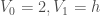 , and
, and  for
for  . Then
  is a square root of modulo .
2. The proof of the Lucas-Lehmer test presented above is due to Michael Rosen, with simplifications by J.W. Bruce. Our exposition was influenced by this blog post written by Terry Tao, which the interested reader should definitely consult.
3. Our “Key Lemma” can also be proved using Galois theory: the Galois group of over has order 2 and both  and
and  are non-trivial automorphisms, so they must coincide.
4. The complexity of Cipolla’s Algorithm is  bit operations, which is asymptotically better than the worst case of Tonelli-Shanks Algorithm. There is no known deterministic polynomial-time algorithm for computing square roots modulo a prime. However, assuming the generalized Riemann hypothesis, it is known that there is a quadratic non-residue less than
  , which makes it possible to determine suitable values of and in Cipolla’s algorithm in polynomial time.
5. Our statement and proof of the main theorem used in the Lucas-Lehmer test is reminiscent of another classical result attributed to Lucas: if and are relatively prime positive integers with  and
and  for all prime divisors of
  , then is prime (and is a primitive root mod ). Lucas viewed this as the correct “converse” to Fermat’s Little Theorem.
6. The Chebyshev polynomial which one iterates in the Lucas-Lehmer test is very special from the point of view of algebraic dynamics (for example, one can explicitly write down its preperiodic points and its Julia set is the real segment ![[-2,2]](https://s0.wp.com/latex.php?latex=%5B-2%2C2%5D&bg=ffffff&fg=404040&s=0&c=20201002) ). I don’t know if this connection has any significance…
). I don’t know if this connection has any significance…
 The French mathematician Edouard Lucas (of Lucas sequence fame) showed in 1876 that the 39-digit Mersenne number
  of 31 University of California faculty members fired for refusing to sign a loyalty oath during the McCarthy era. In 1952, the California Supreme Court declared the oath unconstitutional, and Lehmer returned to Berkeley shortly thereafter. Lehmer also built a number of fascinating mechanical sieve machines designed to factor large numbers.
I updated this post based on helpful comments and corrections by Keith Conrad. Keith pointed out that in the proof of Theorem 2, a little more should be said about the compatibility of the calculation of (2+sqrt(3))^((n+1)/2) in (Z/n)[sqrt(3)], as the theorem requires, and its calculation in the field F, which is carried out only in the proof. I will clarify this in my next post (coming soon!). Keith also noted: “In the 4th observation, this use of GRH is for Dirichlet L-functions. If Dirichlet L-functions were proved to be zero free for Re(s) > 1 – epsilon then the least quadratic nonresidue mod p would be O((log p)^(1/epsilon)), which would make the algorithm polynomial-time as long as there were any vertical strip to the left of Re(s) = 1 that is zero-free for all Dirichlet L-functions.”
Pingback: Lucas sequences and Chebyshev polynomials | Matt Baker's Math Blog
We now link to you
dick